Predicting Drug-Protein Binding Affinity with Graph Neural Networks
Introduction
Drug discovery is expensive and time-consuming. Before a drug candidate reaches clinical trials, researchers must screen thousands of molecules to find those that bind strongly to target proteins. This project explores using machine learning (specifically Graph Neural Networks aka GNNS) to predict binding affinity between proteins and small molecules, potentially accelerating this screening process.
The core question: given a protein sequence and a drug molecule, can we predict how tightly they'll bind?
The Dataset: BindingDB
I used BindingDB, a public database containing millions of measurements of protein-ligand binding affinities. Each entry includes:
- Protein sequence: The amino acid chain (e.g., "MKTAYIAKQR...")
- Ligand (drug) SMILES: A text representation of the molecule's structure
- Kd value: Dissociation constant measuring binding strength (in nanomolar)
The raw dataset is massive (~2GB), so I processed it in chunks of 100,000 rows to avoid memory issues. After filtering for human proteins with valid Kd measurements and protein sequences, I had ~50,000 protein-ligand pairs to work with.
Important preprocessing detail: I converted Kd from nanomolar to molar, then took the negative log to get pKd = -log10(Kd). This makes the scale more interpretable. A higher pKd means stronger binding.
# From src/inspect_BindingDB.py
chunk['Kd_M'] = pd.to_numeric(chunk['Kd (nM)'], errors='coerce') * 1e-9
chunk['pKd'] = -np.log10(chunk['Kd_M'])
Critical Decision: How to Split the Data
Here's where many drug-binding prediction projects fail: the train/test split strategy.
The naive approach: Randomly split all protein-ligand pairs into train (70%), validation (15%), and test (15%). This seems reasonable, right?
The problem: Proteins appear multiple times in the dataset bound to different ligands. If the same protein appears in both training and test sets (with different drugs), your model learns that specific protein's binding properties during training, then "cheats" by recognizing it at test time. Your test performance looks great, but the model won't generalize to truly novel proteins.
The solution: Protein-level splitting. I split by unique proteins, ensuring any protein in the test set never appeared during training.
# From src/split_BindingDB.py
unique_proteins = df['BindingDB Target Chain Sequence 1'].unique()

# Split unique proteins (not individual rows)
train_proteins, temp_proteins = train_test_split(
    unique_proteins,
    test_size=0.3,
    random_state=42
)

val_proteins, test_proteins = train_test_split(
    temp_proteins,
    test_size=0.5,
    random_state=42
)

# Then filter dataframe by protein sets
train_df = df[df['BindingDB Target Chain Sequence 1'].isin(train_proteins)]
This is harder as your model must generalize to completely unseen proteins (but it's the only honest evaluation). This is called stratified splitting, and it's standard practice in bioinformatics ML.
Representing Proteins: ESM-2 Embeddings
Proteins are sequences of amino acids (e.g., "MKTAYIAKQR..."). Neural networks need fixed-size numerical vectors, not variable-length strings.
Enter ESM-2 (Evolutionary Scale Modeling), a protein language model from Meta AI. It's like BERT, but trained on millions of protein sequences instead of text. ESM-2 learned to predict masked amino acids, capturing biological patterns in the process.
I used the facebook/esm2_t30_150M_UR50D model (150 million parameters) to convert each protein sequence into a 640-dimensional embedding vector:
# From src/generate_protein_embeddings.py
from transformers import AutoTokenizer, AutoModel
import torch

modelVariation = "facebook/esm2_t30_150M_UR50D"
tokenizer = AutoTokenizer.from_pretrained(modelVariation)
model = AutoModel.from_pretrained(modelVariation)

device = "cuda" if torch.cuda.is_available() else "cpu"
model = model.to(device)
model.eval()

def getProteinEmbedding(sequence, model, tokenizer, device):
    inputs = tokenizer(sequence, return_tensors="pt", truncation=True, max_length=1024)
    inputs = {k: v.to(device) for k, v in inputs.items()}

    with torch.no_grad():
        outputs = model(**inputs)

    hidden_states = outputs.last_hidden_state
    embedding = hidden_states.mean(dim=1)
    embedding = embedding.cpu().numpy().squeeze()
    return embedding
Each protein now becomes a 640-dimensional vector that captures its structural and functional properties. These embeddings are cached to disk, so I only compute them once.
Representing Ligands: Two Approaches
Ligands (drug molecules) are trickier. They're represented as SMILES strings (Simplified Molecular Input Line Entry System), a compact text notation for chemical structures.
Example SMILES: CC(=O)Oc1ccccc1C(=O)O (this is aspirin!)
I explored two representations:
1. Morgan Fingerprints (Baseline)
Morgan fingerprints are traditional cheminformatics features (2048-bit vectors) indicating the presence of molecular substructures:
# From src/generate_ligand_features.py
from rdkit import Chem
from rdkit.Chem import AllChem
import numpy as np

def getMFP(smiles, radius=2, n_bits=2048):
    mol = Chem.MolFromSmiles(smiles)

    if mol is None:
        return np.zeros(n_bits)

    fp = AllChem.GetMorganFingerprintAsBitVect(mol, radius=radius, nBits=n_bits)

    # Convert to numpy array
    arr = np.zeros(n_bits)
    for i in range(n_bits):
        arr[i] = fp[i]

    return arr
This gives a fixed 2048-dimensional vector per molecule. Simple and fast.
2. Molecular Graphs (GNN Approach)
GNNs can work directly with molecular graphs:
- Nodes: Atoms (with features like element type, charge, hybridization)
- Edges: Chemical bonds (with features like bond type, aromaticity)
Each molecule becomes a graph with variable numbers of atoms and bonds. This preserves the actual molecular structure rather than just substructure fingerprints.
# From src/generate_ligand_graphs.py
from rdkit import Chem

def getAtomFeatures(atom):
    features = []
    atomTypes = ['C', 'N', 'O', 'S', 'F', 'P', 'Cl', 'Br', 'I']
    atomSymbol = atom.GetSymbol()
    for atomType in atomTypes:
        features.append(1 if atom.GetSymbol() == atomType else 0)
    features.append(1 if atomSymbol not in atomTypes else 0)

    features.append(atom.GetDegree())
    features.append(atom.GetFormalCharge())

    hybridizationTypes = [
        Chem.rdchem.HybridizationType.SP,
        Chem.rdchem.HybridizationType.SP2,
        Chem.rdchem.HybridizationType.SP3,
        Chem.rdchem.HybridizationType.SP3D,
        Chem.rdchem.HybridizationType.SP3D2
    ]
    hyb = atom.GetHybridization()
    for hybType in hybridizationTypes:
        features.append(1 if hyb == hybType else 0)

    features.append(1 if atom.GetIsAromatic() else 0)
    features.append(atom.GetTotalNumHs())

    return features


def getBondFeatures(bond):
    features = []
    bondTypes = [
        Chem.rdchem.BondType.SINGLE,
        Chem.rdchem.BondType.DOUBLE,
        Chem.rdchem.BondType.TRIPLE,
        Chem.rdchem.BondType.AROMATIC
    ]
    for bondType in bondTypes:
        features.append(1 if bond.GetBondType() == bondType else 0)

    features.append(1 if bond.GetIsConjugated() else 0)
    features.append(1 if bond.IsInRing() else 0)

    return features


def smilesToGraph(smiles):
    mol = Chem.MolFromSmiles(smiles)
    if mol is None:
        return None

    nodeFeatures = []
    for atom in mol.GetAtoms():
        nodeFeatures.append(getAtomFeatures(atom))
    edgeIndices = []
    edgeFeatures = []

    for bond in mol.GetBonds():
        i = bond.GetBeginAtomIdx()
        j = bond.GetEndAtomIdx()
        edgeIndices.append((i, j))
        edgeIndices.append((j, i))
        bondFeatures = getBondFeatures(bond)
        edgeFeatures.append(bondFeatures)
        edgeFeatures.append(bondFeatures)

    return {
        'nodeFeatures': nodeFeatures,
        'edgeIndex': edgeIndices,
        'edgeFeatures': edgeFeatures,
        'numNodes': len(nodeFeatures),
    }
Model 1: XGBoost Baseline
Before diving into GNNs, I established a baseline using XGBoost (a popular gradient boosting algorithm).
Architecture: Concatenate protein embedding (640-dim) + ligand fingerprint (2048-dim) = 2688-dimensional input vector → XGBoost regressor → pKd prediction
Results:
- Test RMSE: 1.441
- Test R²: 0.163
This gives us a reference point. The model explains ~16% of variance in binding affinity (decent but could def be better).
Model 2: Graph Neural Network
GNNs can learn directly from molecular graphs instead of fixed fingerprints. The architecture has two parts:
Part 1: Ligand Graph Encoder
Converts variable-size molecular graph → 128-dim embedding
# From models/gnn.py
import torch
import torch.nn as nn
import torch.nn.functional as F

class GraphConvolutionLayer(nn.Module):

    def __init__(self, inFeatures, outFeatures):
        super(GraphConvolutionLayer, self).__init__()
        self.linear = nn.Linear(inFeatures, outFeatures)
        self.edgeLinear = nn.Linear(6, outFeatures)  # 6-dim edge features

    def forward(self, nodeFeatures, edgeIndex, edgeFeatures):
        numNodes = nodeFeatures.size(0)
        transformed = self.linear(nodeFeatures)
        aggregated = torch.zeros(numNodes, transformed.size(1), device=nodeFeatures.device)
        for idx, (src, dst) in enumerate(edgeIndex):
            edgeMessage = self.edgeLinear(edgeFeatures[idx])
            aggregated[dst] += transformed[src] + edgeMessage
        return F.relu(aggregated)
The GNN encoder stacks multiple graph convolution layers, letting information flow through the molecular graph. After 3-4 layers, we pool all atom embeddings (via mean pooling) to get a single 128-dim vector representing the entire molecule.
Part 2: Binding Affinity Predictor
Concatenate protein embedding (640-dim) + ligand graph embedding (128-dim) → MLP → pKd prediction
# From models/gnn.py
class BindingAffinityGNN(nn.Module):

    def __init__(self, proteinDimension=640, ligandGnnOutput=128, hiddenDimension=256):
        super(BindingAffinityGNN, self).__init__()
        self.ligandEncoder = GNNEncoder(
            nodeFeaturesDimension=19,
            hiddenDimension=128,
            outputDimension=ligandGnnOutput,
            numLayers=3
        )
        combinedDimension = proteinDimension + ligandGnnOutput
        self.mlp = nn.Sequential(
            nn.Linear(combinedDimension, hiddenDimension),
            nn.ReLU(),
            nn.Dropout(0.3),

            nn.Linear(hiddenDimension, hiddenDimension // 2),
            nn.ReLU(),
            nn.Dropout(0.3),

            nn.Linear(hiddenDimension // 2, 1)
        )

    def forward(self, proteinEmbedding, nodeFeatures, edgeIndex, edgeFeatures):
        ligandEmbedding = self.ligandEncoder(nodeFeatures, edgeIndex, edgeFeatures)
        combined = torch.cat([proteinEmbedding, ligandEmbedding], dim=0)
        prediction = self.mlp(combined)

        return prediction
Model Iterations & Results
I trained several GNN variants, tweaking architecture and regularization:
| Model | Test RMSE | Test R² | Key Changes |
|---|---|---|---|
| XGBoost | 1.441 | 0.163 | Baseline (concatenated features) |
| GNN | 1.510 | 0.081 | Initial 4-layer GNN |
| GANN | 1.506 | 0.086 | Added attention pooling (overfitted) |
| GNN Iter3 | 1.425 | 0.182 | 4 layers + residual connections + batch norm |
| GNN Iter4 | 1.464 | 0.137 | 3 layers + residuals |
| GNN Iter5 | 1.495 | 0.100 | 3 layers + gradient clipping |
Best performer: GNN Iter3 with RMSE of 1.425 and R² of 0.182.
What Worked:
- Residual connections: Help gradients flow through deep GNN layers
- Batch normalization: Stabilized training
- Dropout (0.2-0.3): Prevented overfitting
What Didn't Work:
- Attention pooling (GANN): Overfitted-validation loss diverged from training
- Too many layers: Diminishing returns beyond 4 GNN layers
- Aggressive gradient clipping: Slowed learning without improving generalization
Visualizing Results
Model Comparison
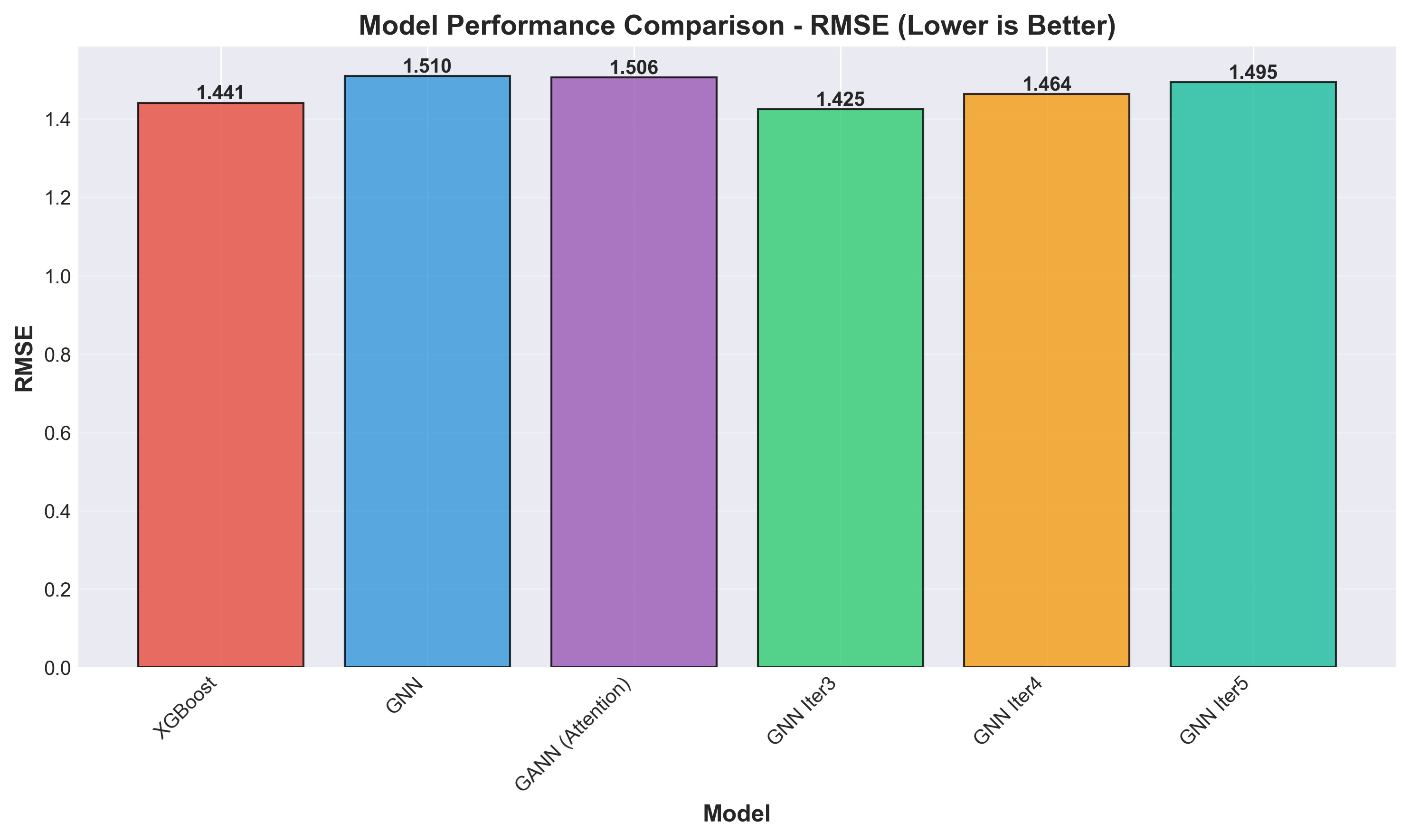 Lower RMSE is better. GNN Iter3 achieves the lowest error
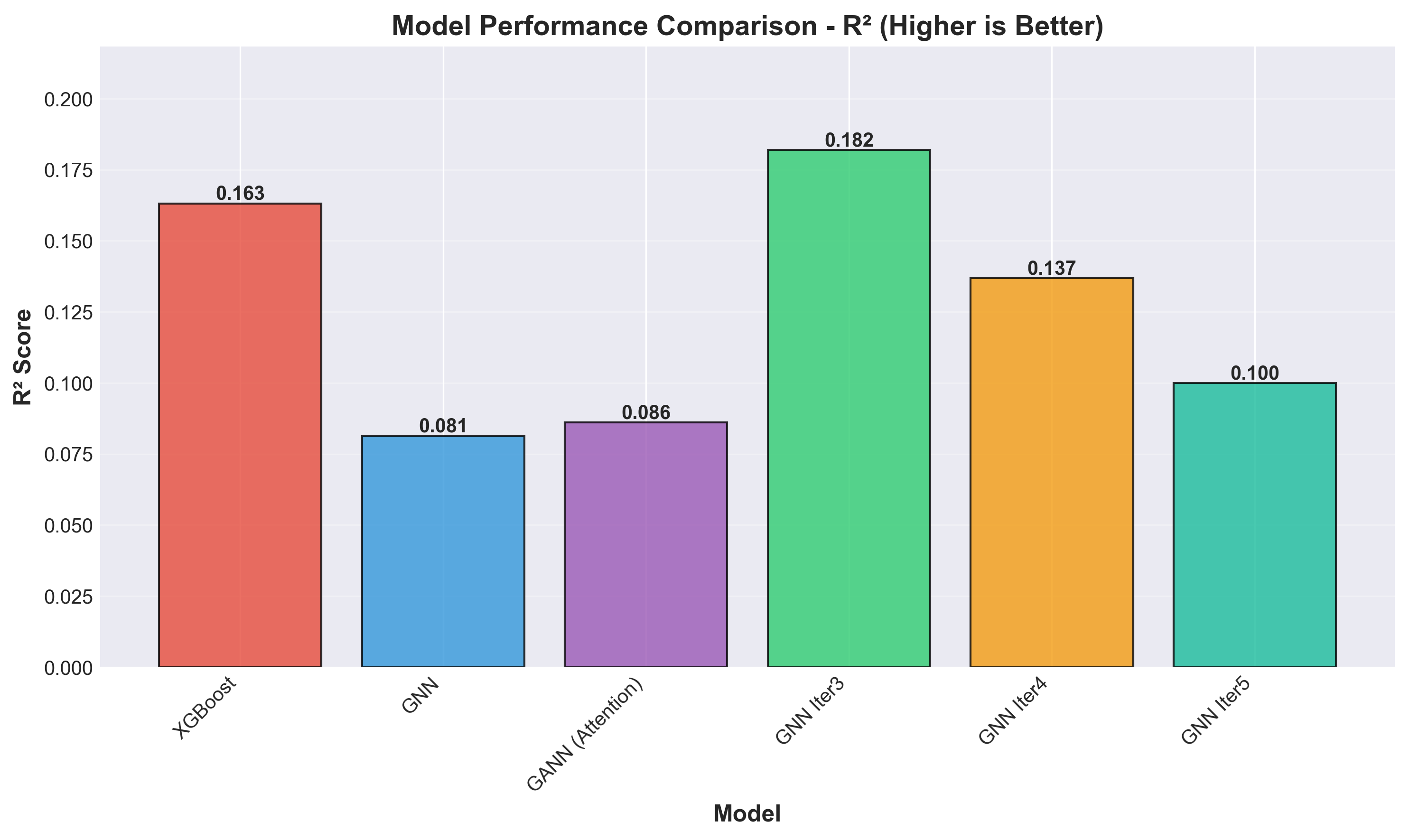 R2 indicates the variance. Higher is better
Data Distribution
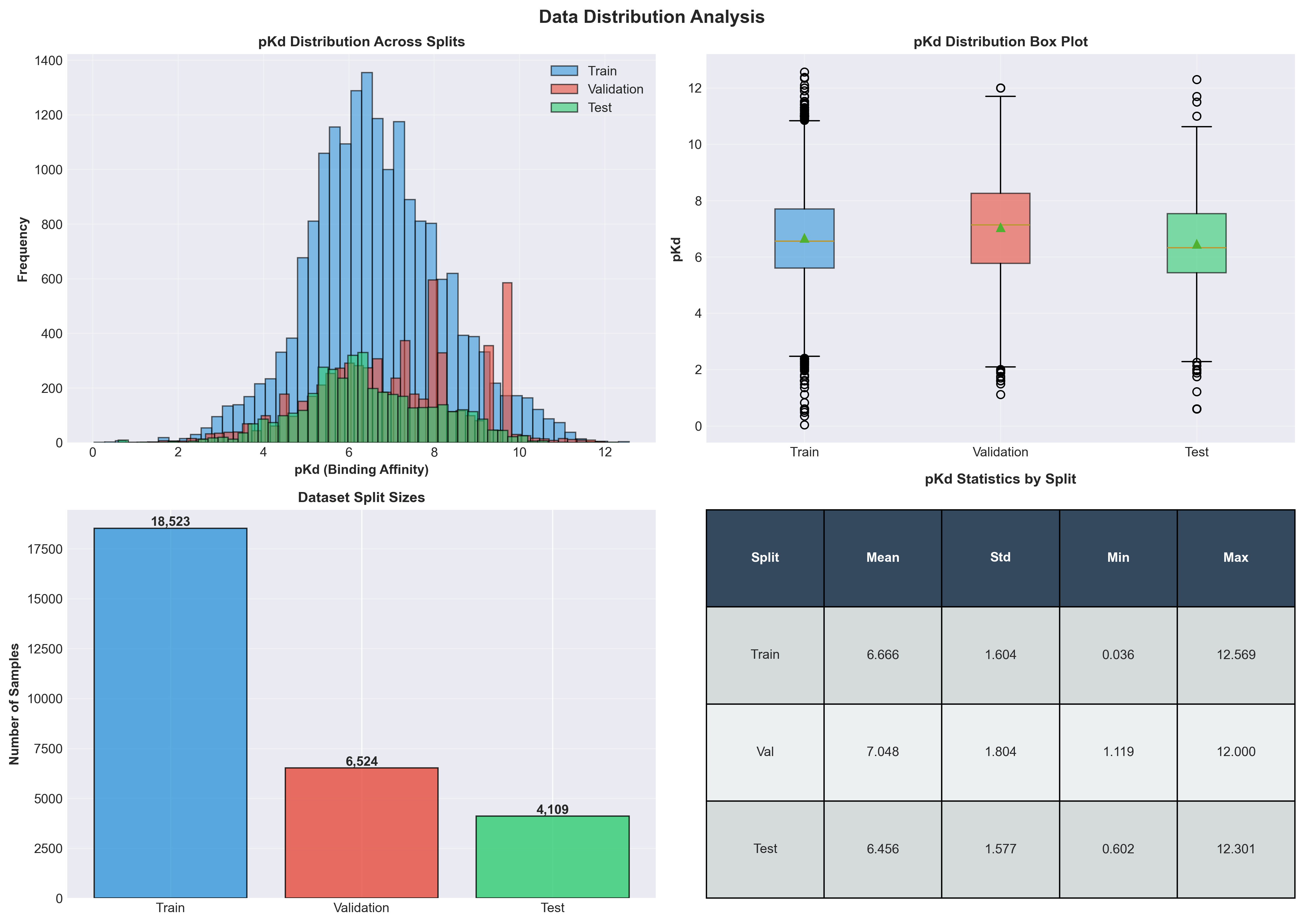 Illustration of data
Key Takeaways
-
GNNs are effective for molecular data: GNN Iter3 outperformed the XGBoost baseline, showing that graph structure carries useful information beyond molecular fingerprints.
-
Proper data splitting is crucial: Protein-level splitting prevents data leakage but makes the problem harder. Random splitting would give inflated performance that doesn't generalize.
-
Architecture choices matter: Residual connections and batch normalization made the difference between GNN Iter3 (best) and the original GNN (worst performer).
-
Modest improvements, hard problem: Even the best model (R² = 0.182) explains less than 20% of variance. Binding affinity depends on many factors beyond sequence and structure, such as 3D protein conformation, solvent effects, temperature, etc. This is a genuinely difficult prediction task.
-
Transfer learning helps: Using pre-trained ESM-2 for protein embeddings was essential. Training protein encoders from scratch would require far more data.
Future Directions
- 3D protein structure: Incorporate AlphaFold-predicted structures instead of just sequences
- Attention mechanisms: Properly implemented cross-attention between protein and ligand
- Larger datasets: BindingDB has millions of entries (I only used ~50k)
- Multi-task learning: Predict other properties (Ki, IC50) jointly
- Uncertainty quantification: Add probabilistic predictions to flag uncertain cases
Conclusion
Predicting drug-protein binding affinity is challenging, but Graph Neural Networks show promise for learning from molecular structure. The project reinforced that successful ML in drug discovery requires both sophisticated models AND rigorous experimental design. Fancy architectures won't save you from data leakage.
The code and visualizations are available on GitHub.